Materialization
So far, we executed our dataflow using the Driver.execute() method, which can receive an inputs dictionary and return a results dictionary (by default). However, you can also execute code with Driver.materialize() to directly read from / write to external data sources (file, database, cloud data store).
On this page, you’ll learn:
How to load and save data in Apache Hamilton
Why use materialization
What are
DataSaverandDataLoaderobjectsThe difference between
.execute()and.materialize()The basics to write your own materializer
Different ways to write the same dataflow
Below are 6 ways to write a dataflow that:
loads a dataframe from a parquet file
preprocesses the dataframe
trains a machine learning model
saves the trained model
The first two options don’t use the concept of materialization and the next four do.
Without materialization
|
|
|---|---|
import pandas as pd
import xgboost


def raw_df(data_path: str) -> pd.DataFrame:
    """Load raw data from parquet file"""
    return pd.read_parquet(data_path)


def preprocessed_df(raw_df: pd.DataFrame) -> pd.DataFrame:
    """preprocess raw data"""
    return ...


def model(preprocessed_df: pd.DataFrame) -> xgboost.XGBModel:
    """Train model on preprocessed data"""
    return ...


def save_model(model: xgboost.XGBModel, model_dir: str) -> None:
    """Save trained model to JSON format"""
    model.save_model(f"{model_dir}/model.json")


if __name__ == "__main__":
    import __main__

    from hamilton import driver

    dr = driver.Builder().with_modules(__main__).build()

    data_path = "..."
    model_dir = "..."
    inputs = dict(data_path=data_path, model_dir=model_dir)
    final_vars = ["save_model"]
    results = dr.execute(final_vars, inputs=inputs)
    # results["save_model"] == None
|
import pandas as pd
import xgboost


def preprocessed_df(raw_df: pd.DataFrame) -> pd.DataFrame:
    """preprocess raw data"""
    return ...


def model(preprocessed_df: pd.DataFrame) -> xgboost.XGBModel:
    """Train model on preprocessed data"""
    return ...


if __name__ == "__main__":
    import __main__

    from hamilton import driver

    dr = driver.Builder().with_modules(__main__).build()

    data_path = "..."
    model_dir = "..."
    inputs = dict(raw_df=pd.read_parquet(data_path))
    final_vars = ["model"]

    results = dr.execute(final_vars, inputs=inputs)
    results["model"].save_model(f"{model_dir}/model.json")
|
|
|
Observations:
These two approaches load and save data using
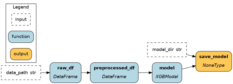
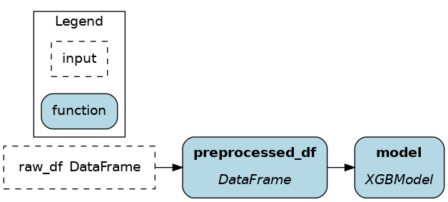
pandasandxgboostwithout any Apache Hamilton constructs. These methods are transparent and simple to get started, but as the number of node grows (or across projects) defining one node per parquet file to load introduces a lot of boilerplate.Using 1) from nodes improves visibility by including loading & saving in the dataflow (as illustrated).
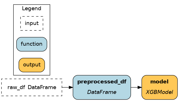
Using 2) from ``Driver`` facilitates modifying loading & saving before code execution when executing the code, without modifying the dataflow itself. It is particularly useful when moving from development to production.
Limitations
Apache Hamilton’s approach to “materializations” aims to solve 3 limitations:
Redundancy: deduplicate loading & saving code to improve maintainability and debugging
Observability: include loading & saving in the dataflow for full observability and allow hooks
Flexibility: change the loading & saving behavior without editing the dataflow
With materialization
|
|
|
|
|---|---|---|---|
import pandas as pd
import xgboost

from hamilton.function_modifiers import dataloader, datasaver
from hamilton.io import utils


@dataloader()
def raw_df(data_path: str) -> tuple[pd.DataFrame, dict]:
    """Load raw data from parquet file"""
    df = pd.read_parquet(data_path)
    return df, utils.get_file_and_dataframe_metadata(data_path, df)


def preprocessed_df(raw_df: pd.DataFrame) -> pd.DataFrame:
    """preprocess raw data"""
    return ...


def model(preprocessed_df: pd.DataFrame) -> xgboost.XGBModel:
    """Train model on preprocessed data"""
    return ...


@datasaver()
def save_model(model: xgboost.XGBModel, model_dir: str) -> dict:
    """Save trained model to JSON format"""
    model.save_model(f"{model_dir}/model.json")
    return utils.get_file_metadata(f"{model_dir}/model.json")


if __name__ == "__main__":
    import __main__

    from hamilton import driver

    dr = driver.Builder().with_modules(__main__).build()
    data_path = "..."
    model_dir = "..."
    inputs = dict(data_path=data_path, model_dir=model_dir)
    final_vars = ["save_model"]
    results = dr.execute(final_vars, inputs=inputs)
    # results["save_model"] == None
|
import pandas as pd
import xgboost


def preprocessed_df(raw_df: pd.DataFrame) -> pd.DataFrame:
    """preprocess raw data"""
    return ...


def model(preprocessed_df: pd.DataFrame) -> xgboost.XGBModel:
    """Train model on preprocessed data"""
    return ...


if __name__ == "__main__":
    import __main__

    from hamilton import driver
    from hamilton.io.materialization import from_, to

    data_path = "..."
    model_dir = "..."
    materializers = [
        from_.parquet(target="raw_df", path=data_path),
        to.json(
            id="model__json",  # name of the DataSaver node
            dependencies=["model"],
            path=f"{model_dir}/model.json",
        ),
    ]
    dr = (
        driver.Builder()
        .with_modules(__main__)
        .with_materializers(*materializers)
        .build()
    )

    results = dr.execute(["model", "model__json"])
    # results["model"]  <- the model
    # results["model__json"] <- metadata from saving the model
|
import pandas as pd
import xgboost


def preprocessed_df(raw_df: pd.DataFrame) -> pd.DataFrame:
    """preprocess raw data"""
    return ...


def model(preprocessed_df: pd.DataFrame) -> xgboost.XGBModel:
    """Train model on preprocessed data"""
    return ...


if __name__ == "__main__":
    import __main__

    from hamilton import driver
    from hamilton.io.materialization import from_, to

    data_path = "..."
    model_dir = "..."
    materializers = [
        from_.parquet(target="raw_df", path=data_path),
        to.json(
            id="model__json",  # name of the DataSaver node
            dependencies=["model"],
            path=f"{model_dir}/model.json",
        ),
    ]
    dr = driver.Builder().with_modules(__main__).build()
    # executes all `to.` materializers; use `additional_vars` to execute other nodes
    metadata, results = dr.materialize(*materializers, additional_vars=["model"])
    # results["model"]  <- the model
    # metadata["model__json"] <- metadata from saving the model
|
import pandas as pd
import xgboost

from hamilton.function_modifiers import load_from, save_to, source


# source("data_path") allows to read the input value for `data_path`
@load_from.parquet(path=source("data_path"))
def preprocessed_df(raw_df: pd.DataFrame) -> pd.DataFrame:
    """preprocess raw data"""
    return ...


@save_to.json(path=source("model_path"))
def model(preprocessed_df: pd.DataFrame) -> xgboost.XGBModel:
    """Train model on preprocessed data"""
    return ...


if __name__ == "__main__":
    import __main__

    from hamilton import driver

    dr = driver.Builder().with_modules(__main__).build()

    data_path = "..."
    model_path = "..."
    inputs = dict(data_path=data_path, model_path=model_path)
    final_vars = ["save.model", "model"]
    results = dr.execute(final_vars, inputs=inputs)
    # results["model"]  <- the model
    # results["save.model"] <- metadata from saving the model
|
|
|
|

|
Simple Materialization
When you don’t need to hide the implementation details of how you read and write, but you want to track what was read and written, you need to expose extra metadata. This is where the @datasaver() and @dataloader() decorators come in. They allow you to return metadata about what was read and written, and this metadata is then used to track what was read and written.
This is our recommended first step when you’re starting to use materialization in Apache Hamilton.
Static materializers
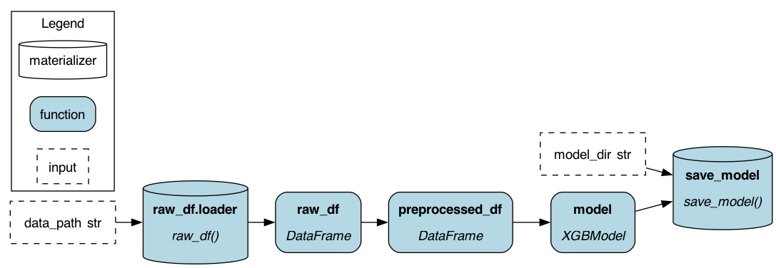
Passing from_ and to Apache Hamilton objects to Builder().with_materializers() injects into the dataflow standardized nodes to load and save data. It solves the 3 limitations highlighted in the previous section:
Redundancy ✅: Using the
from_andtoApache Hamilton constructs reduces the boilerplate to load and save data from common formats (JSON, parquet, CSV, etc.) and to interact with 3rd party libraries (pandas, matplotlib, xgboost, dlt, etc.)Observability ✅: Loaders and savers are part of the dataflow. You can view them with
Driver.display_all_functions()and execute nodes by requesting them withDriver.execute().Flexibility ✅: The loading and saving behavior is decoupled from the dataflow and can modified easily when creating the
Driverand executing code.
Note
from_ data loaders can be specified as optional with optional=True. This allows specified data loaders to be skipped rather than raise an exception when not referenced by a dataflow.
Dynamic materializers
The dataflow is executed by passing from_ and to objects to Driver.materialize() instead of the regular Driver.execute(). This approach ressembles 2) from Driver:
Note
Driver.materialize() can receive data savers (from_) and loaders (to) and will execute all to passed. Like Driver.execute(), it can receive inputs, and overrides, but instead of final_vars it receives additional_vars.
Redundancy ✅: Uses
from_andtoApache Hamilton constructs.Observability 🚸: Materializers are visible with
Driver.visualize_materialization(), but can’t be introspected otherwise. Also, you need to rely onDriver.materialize()which has a different call signature.Flexibility ✅: Loading and saving is decoupled from the dataflow.
Note
Using static materializers is typically preferrable. Static and dynamic materializers can be used together with dr = Builder.with_materializers().build() and later dr.materialize().
Function modifiers
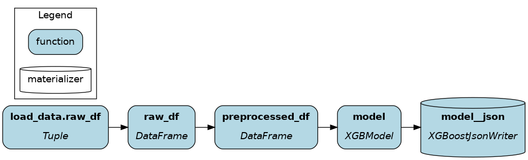
By adding @load_from and @save_to function modifiers (Load and save external data) to Hamilton functions, materializers are generated when using Builder.with_modules(). This approach ressembles 1) from Driver:
Note
Under the hood, the @load_from modifier uses the same code as from_ to load data, same for @save_to and to.
Redundancy 🚸: Using
@load_fromand@save_toreduces redundancy. However, to make available to multiple nodes a loaded table, you would need to decorate each node with the same@save_to. Also, it might be impractical to decorate dynamically generated nodes (e.g., when using the@parameterizefunction modifier).Observability ✅: Loaders and savers are part of the dataflow.
Flexibility 🚸: You can modify the path and materializer kwargs at runtime using
source()in the decorator definition, but you can’t change the format itself (e.g., from parquet to CSV).
Note
It can be desirable to couple loading and saving to the dataflow using function modifiers. It makes it clear when reading the dataflow definition which nodes should load or save data using external sources.
DataLoader and DataSaver
In Apache Hamilton, DataLoader and DataSaver are classes that define how to load or save a particular data format. Calling Driver.materialize(DataLoader(), DataSaver()) adds nodes to the dataflow (see visualizations above).
Here are simplified snippets for saving and loading an XGBoost model to/from JSON.
DataLoader
DataSaver
To define your own DataSaver and DataLoader, the Apache Hamilton XGBoost extension provides a good example
SQL metadata and lineage
The built-in SQL materializers (@load_from.sql, @save_to.sql, from_.sql, to.sql and the
PandasSqlReader / PandasSqlWriter behind them) return sql_metadata describing what was read
or written. Since version 1.1.0 of that metadata, they also record where: the database the
connection points at. Lineage consumers such as the OpenLineage adapter use this to name the physical tables a query
reads, without any custom loader or hand-maintained mapping.
Take a graph that reads a query joining orders and customers from a sales database,
aggregates daily revenue in Python, and writes daily_revenue to a reporting database:
@load_from.sql(query_or_table=value(REVENUE_QUERY), db_connection=source("sales_db"))
def order_lines(df: pd.DataFrame) -> pd.DataFrame:
    return df

@save_to.sql(table_name=value("daily_revenue"), schema=value("reporting"),
             db_connection=source("warehouse_db"), output_name_="saved_revenue")
def daily_revenue(order_lines: pd.DataFrame) -> pd.DataFrame:
    ...
With metadata version 1.0.0, the loader’s metadata was {"rows": 3, "query": "...", "table_name": None}: no table, no
server, no database. A join reported no inputs at all, and the saver’s daily_revenue could not
be told apart from a table of the same name elsewhere. With version 1.1.0, the same code, with the same
connections, yields:
{"sql_metadata": {
    "rows": 3,
    "query": "WITH paid AS (...) SELECT ... FROM paid p JOIN customers c ON ...",
    "table_name": None,
    "schema": None,
    "operation": "read",
    "source": {"dialect": "postgresql", "host": "source.example", "port": 5432,
               "database": "sales", "default_schema": "public"},
    "notes": "",
    "timestamp": 1758470400.0,
    "__version__": "1.1.0",
}}
and the OpenLineage adapter, with sql_dataset_identity="datasource" (see
Migrating to the datasource identity), reports sales.public.orders and sales.public.customers under
postgres://source.example:5432 as inputs, and analytics.reporting.daily_revenue under the
warehouse’s namespace as output. The same module produces the same identities whether it runs from
a script, a notebook or an orchestrator.
Fields
The sql_metadata entry holds the following keys:
Key |
Meaning |
|---|---|
|
Rows read ( |
|
The statement executed, or |
|
The bare table name read or written, or |
|
The schema explicitly passed to the writer ( |
|
|
|
The datasource, or |
|
Why |
|
When the metadata was produced (POSIX seconds). |
|
|
Supported connections
The connection object determines what source can hold:
Connection passed as |
What |
|---|---|
SQLAlchemy |
dialect, host, port, database from the URL; |
SQLAlchemy URL string ( |
dialect, host, port, database from the parsed URL; |
Standard-library |
|
In-memory SQLite ( |
|
Anything else (other DBAPI connections, mocks, and similar objects) |
|
Inspection never opens a connection, runs a write, commits, rolls back, or changes session settings,
and never raises: a failure during inspection becomes a notes entry naming the exception type
only. source holds scalars, never the connection object or the URL string, so it serializes
with json.dumps and cannot carry a username, password or URL query parameter. The query
field is the SQL text you supplied, as before: keep secrets out of literals or strip them
downstream.
Schema precedence and unknown cases
A table referenced by a statement is qualified from, in order: the qualification written in the
SQL (sales.public.orders), the schema argument given to the writer, then source["default_schema"].
For SQLite, a schema names a database file rather than a namespace inside one: main (or no
schema) is the connection’s file, and an attached database’s tables are named in that file’s
namespace, resolved through source["attached"]. When the attached file cannot be known (a URL
or SQLAlchemy connection), or the schema is temp, the table is left out rather than
attributed to the main file.
The default schema is what SQLAlchemy read from the server, not an assumption that PostgreSQL uses
public; when the connection’s search_path spans several schemas, qualify table names in
the SQL to remove the ambiguity. When no schema can be determined, the table is left out of
lineage and the reason is reported. Only SELECT-style statements pandas can execute are in
scope; SQL run inside ordinary Python functions is not observed.
Call the helper yourself
Custom @dataloader / @datasaver functions can produce the same metadata:
from hamilton.io import utils

@dataloader()
def orders(sales_db: Engine) -> tuple[pd.DataFrame, dict]:
    query = "SELECT * FROM sales.public.orders"
    df = pd.read_sql(query, sales_db)
    return df, utils.get_sql_metadata(query, df, db_connection=sales_db, operation="read")
Pass operation="write" from a saver so the table name is never mistaken for a statement.
The original two-argument call get_sql_metadata(query_or_table, results) keeps working and
keeps its keys, their values and row-count semantics; it simply reports source=None with a note and
operation=None, so consumers diagnose it as incomplete rather than guessing.